



 Multi-industry nationwide coverage (municipal wastewater treatment / centralized
 Pilot to full-scale engineering (tens of thousands to 120,000 m³/d; hundreds to
Aerators: The Efficiency on the Nameplate Is Measured in a Clean Water Tank
The same aerator, on a clean-water test bench it is 26%, but in your tank it is only 10.4%. In between lie two coefficients, α and F, and neither is printed on the datasheet.
Aeration is the core of the Activated Sludge process and the largest single electricity consumer in a wastewater treatment plant. During selection, almost everyone looks at the single number "oxygen transfer efficiency," yet rarely asks: under what water, what temperature, what depth, new membrane or old membrane conditions was this number measured? The answer is usually — clean water, 20℃, 0.1 MPa, brand-new membrane. It belongs to the test bench, not to your tank. This article peels apart, layer by layer, the several discounts that take the aeration system from the "datasheet number" to the "field number," and restores the seemingly one-step calculation of "how many aerators are actually needed" to what it really is: two calculation methods, and the parameters of both methods are themselves ranges.
I. First, how big is this "power hog" really: one share, six ways of counting
The statement "aeration accounts for 50%~70% of wastewater treatment plant energy consumption" has been cited so many times that few notice it is actually a range in which six definitions coexist. The difference is not measurement error but three things: whether the denominator is "whole-plant electricity consumption" or "biological treatment stage energy consumption"; whether the measure is "electricity consumption" or "broad-sense energy consumption (including heat)"; and whether what is counted is "measured equipment data" or "industry estimates."
| Value | Denominator | Source type |
|---|---|---|
| 45%~75% | Total energy consumption of the wastewater treatment plant | Journal paper abstract (study on membrane pore parameters and surfactants) |
| 50%~70% | Total electricity consumption of the wastewater treatment plant | Multiple equipment manufacturers and industry media, cited in data from the China Urban Water Association |
| 50%~65% | Net power demand of the wastewater treatment plant | US EPA 832-F-99-065 (1999) |
| 50%~80% | Share of plant-wide energy consumption accounted for by the biological treatment stage | Xylem technical documentation (2019—2022) |
| 58% / 25% / 12% | Measured three-part breakdown at a 10 万 m³/d wastewater treatment plant (aeration / lifting pumps / sludge treatment) | Plant measurements as reported by industry media |
| 2%~5% | Share of capital investment accounted for by the aeration system (not energy consumption) | Industry technical documentation |
Note: The last row is not an energy-consumption basis; it is listed separately because it is often used to argue that "aeration is not worth investing in for retrofitting" — a small share of capital investment and a large share of operating consumption are simply two sides of the same coin.
What this table is really saying is: when someone says "aeration accounts for seventy percent," you first need to ask them: seventy percent of what. Taking "the biological treatment stage accounts for 50%~80%" and directly citing it as "the whole plant accounts for 50%~80%" will systematically overestimate the aeration bill, and in turn underestimate the 25% of room in the pipe network and lift pumps.
II. "Oxygen Transfer Efficiency" Has Five Names and Three Dimensions
When the industry says "oxygen transfer efficiency," it may refer to five completely different metrics. They have different dimensions, different test conditions, and can answer different questions, and they cannot be converted into one another. The most common mistake is to take the SOTE from a sample, directly divide it by the air flow rate, and then multiply by an "efficiency" to use as the on-site oxygen consumption—that chain breaks at the very first step.
| Indicator | Dimension | What It Answers |
|---|---|---|
| SOTR (Standard Oxygen Transfer Rate) | kgO₂/h | How much oxygen one aerator can transfer per hour under standard conditions—the intrinsic capability of the equipment |
| SOTE (Standard Oxygen Transfer Efficiency) | % (can be expressed as overall %, or as %/m normalized by water depth) | What proportion of the oxygen in the supplied air dissolves into the water—the efficiency of the air supply system |
| SSOTE (Specific Standard Oxygen Transfer Efficiency) | %·m⁻¹ | SOTE divided by submergence depth, facilitating comparison across different tank depths—for comparison, not for design |
| OTE (Field Oxygen Transfer Efficiency) | % | How much actually dissolves into your tank—for operational diagnostics |
| SAE (Standard Aeration Efficiency / Power Efficiency) | kgO₂/kWh | How much oxygen is obtained per kilowatt-hour—an indicator that can be directly converted into electricity costs |
Here is a pitfall that is easily overlooked: SOTE only applies to pressurized air supply systems (diffused aeration). Surface aerators and jet aerators do not report figures on this basis; they directly provide SAE. Putting the SOTE of these two types of equipment into the same price comparison table is equivalent to comparing numbers from two different languages side by side.
SAE, on the other hand, is the one that shows up on the electricity bill. Publicly available benchmark values are roughly as follows: optimally designed fine-bubble aeration 2.5~5.0 kgO₂/kWh (equivalent to 0.20~0.40 kWh/kgO₂), an average-performing fine-bubble system 1.8~3.5, coarse-bubble 1.2~2.0, low-speed surface aerators 1.2~2.5, high-speed surface aerators 0.8~1.5, jet aeration 1.0~2.0, and deep-shaft aeration above 15 m at 3.5~6.0. The criterion is simple: if the measured SAE of a fine-bubble aeration system is below 1.8 kgO₂/kWh, that is a recoverable performance problem, usually pointing to one of three causes: membrane fouling, the blower operating away from its high-efficiency range, or the dissolved oxygen setpoint being set too high.
III. The overlooked premise: 0.1 MPa, 20℃, clean water
The Code for Design of Outdoor Wastewater Engineering states this plainly when discussing oxygen supply facilities (clause 6.8.3 explanatory note): the same aerator performs differently under different pressures, different water temperatures, and different water qualities. The oxygen transfer performance data of an aerator refer to the value of a single aerator under standard conditions, i.e., 0.1 MPa, 20℃, clean water. The purpose of this provision is also clear — the oxygen demand of wastewater in a biological reaction tank is not the oxygen demand of clean water; in order to calculate the number of aerators, the oxygen demand of the wastewater must first be converted to the value under standard conditions.
In other words: the conversion step required by the standard is itself an acknowledgment that "the catalog value does not equal the field value." The clean-water test procedure is also printed in the standard method — dosing anhydrous sodium sulfite for deoxygenation, using cobalt chloride as a catalyst, continuously recording dissolved oxygen at no fewer than three sampling points in the tank, waiting until saturation rises from about 10% to above 90%, then using nonlinear regression to determine the overall oxygen transfer coefficient KLa, and finally correcting to standard conditions by temperature and pressure. The entire chain is completed in water that has been deliberately "cleaned up."
IV. Two sets of numbers for the same thing: SOTE "per metre" and "overall" are not the same
This is the first place where a real calculation error occurs. SOTE has two expressions: one is the "per metre" value normalized by submergence depth (%/m, often written in English literature as per metre of submergence), and the other is the total efficiency of the whole tank (overall %). The two are not related by simple multiplication, because during bubble rise the oxygen partial pressure of the gas-liquid two phases and the contact time are both changing, and efficiency is not linear along the depth. More importantly, even for the "per metre" expression, there are two conflicting sets of numbers in the public literature:
| Source basis | Fine-bubble aeration | Coarse-bubble aeration |
|---|---|---|
| Category A (e.g., American Aeration technical articles) | 2.0~4.0 %/m | 0.5~1.0 %/m |
| Category B (e.g., industry design guidelines, equipment technical articles) | 5~7 %/m, some write 6~8 %/m | 2~3 %/m, some write 3~4 %/m |
| Whole-basin overall efficiency (deep basin, common 4~6 m submergence depth) | 25%~40% | about 8%~12% (about one third of fine-bubble) |
Multiplying the Category B 5~7 %/m by 4~6 m lands right around the whole-basin 25%~40%, which is logically self-consistent; multiplying the Category A 2~4 %/m by 4~6 m gives only 10%~20%, which does not match the deep-basin whole-basin data. So the two sets of figures are most likely different definitions of the same thing or different water-depth segments—but the sources almost never state which one is being used.
Comparing how domestic equipment samples are written makes this easier to understand: common domestic disc diffuser samples state "Oxygen Transfer Efficiency (water depth 3.2 m) 18.4%~27.7%%" and "Oxygenation Power Efficiency 4.46~5.19 kgO₂/kWh", where 18.4%~27.7% is the whole-basin efficiency rather than a per-meter value; and for the same type of product, "clean water at 6 m water depth SOTE can reach 30%~38%, power efficiency 7~8.5" also confirms that "the deeper, the higher, but not a linear superposition" — for every 1 m increase in water depth, the oxygen transfer efficiency rises by roughly 4~6 percentage points, rather than simply multiplying the per-meter value by the number of meters.
V. The first discount is α: the finer the bubbles, the harsher this cut
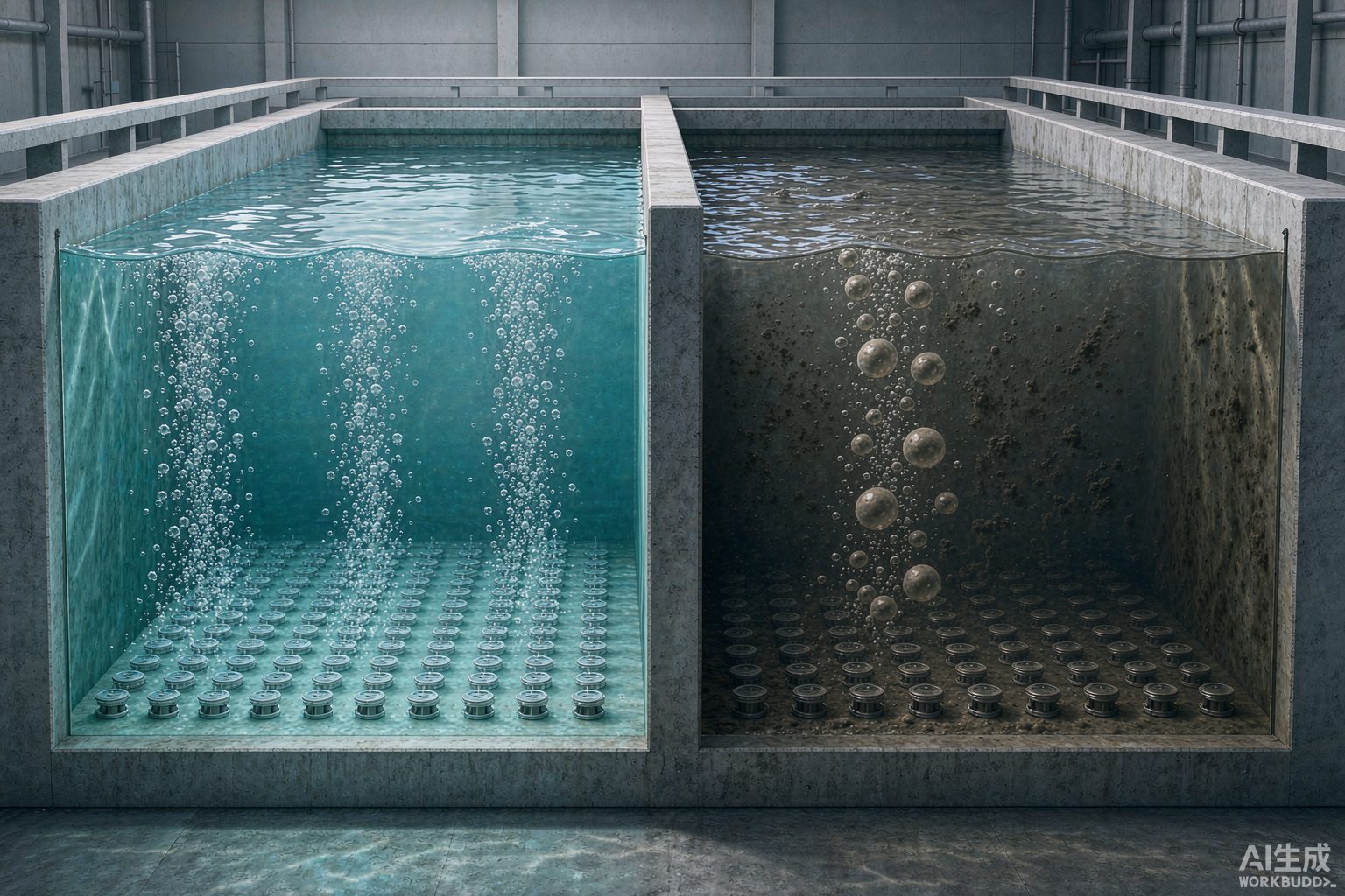
Moving from clean water to wastewater, the first coefficient to multiply by is α (alpha), defined as the ratio of the overall oxygen transfer coefficient in wastewater to that in clean water (KLa wastewater ÷ KLa clean water). It is jointly determined by surfactants, grease, and suspended solids — surfactant molecules migrate to the gas-liquid interface of the bubbles, forming a "skin" that hinders oxygen molecules from passing through.
Here is a counterintuitive rule, and also the sentence most worth remembering in this article: the finer the bubbles, the lower the α.
The reason is that microbubbles have a large specific surface area, rise slowly, and last long, giving surfactants more time to "wrap" them; coarse bubbles are highly turbulent and have short residence times, and are therefore less sensitive to contamination. As a result, the advantage of fine-bubble aeration in clean water is eaten away substantially in wastewater: a system with a clean-water SOTE as high as 2.5 times that of coarse-bubble systems often retains only about one-third of the advantage in an actual basin.
| Factor | What It Corrects | Published Value Range |
|---|---|---|
| α | Reduction of oxygen transfer in wastewater relative to clean water | Fine bubble 0.4~0.8; coarse bubble 0.6~0.9 (other sources give fine bubble 0.4~0.65 vs. coarse bubble 0.6~0.85) |
| β | Effect of dissolved solids on saturated dissolved oxygen | 0.90~0.98 |
| F | Fouling reduction of the membrane over its entire service life | 0.6~0.9 (other sources give 0.8~0.9) |
| θ (temperature correction) | Effect of temperature on mass transfer rate, θ^(T−20) | 1.024 (consistent across sources) |
There is another chemical-level detail about α: pilot studies found that when anionic surfactants (such as sodium dodecylbenzene sulfonate, SDBS) vary within the range of 0~20 mg/L, the overall oxygen transfer coefficient KLa first decreases and then increases—at very low concentrations, the interfacial film forms first and mass transfer deteriorates; as the concentration continues to rise, bubble diameter is compressed smaller and interfacial viscoelasticity changes, so mass transfer recovers instead. This explains why, for the same tank, α does not change monotonically when influent water quality fluctuates; using a single α value on site for precise aeration control inherently has an error boundary.
VI. The second discount is F: fouling turns "micropores" into "coarse pores"
Membrane fouling is divided into two categories in engineering, with completely different mechanisms and different countermeasures:
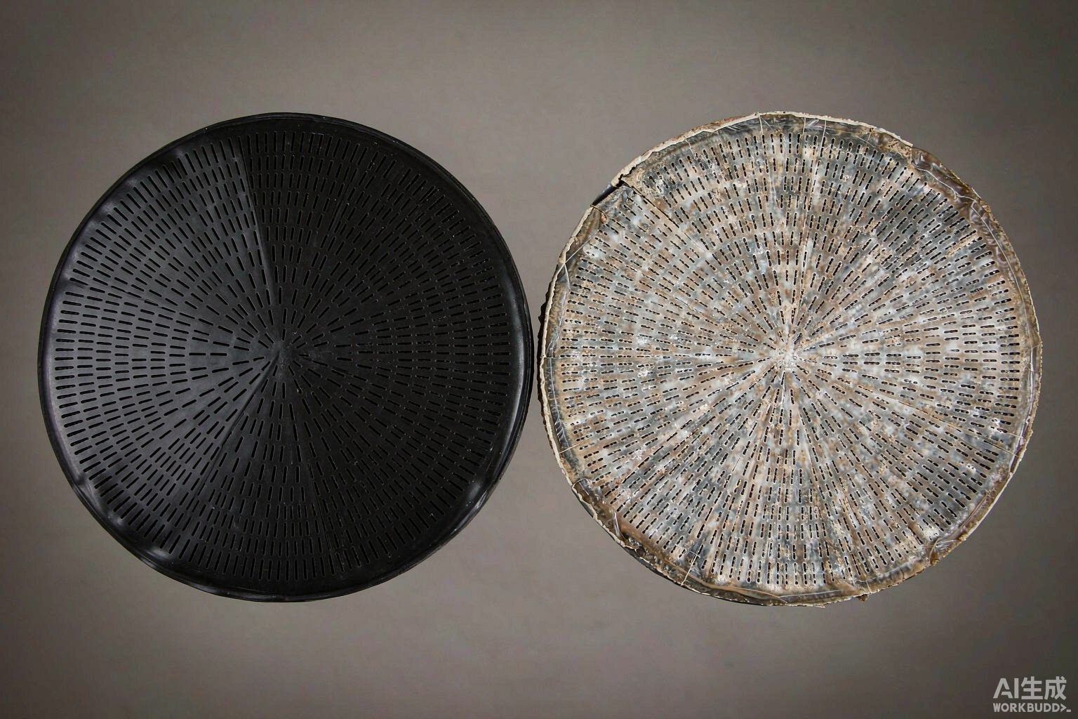
The first category is inorganic scaling (Type I). Salts of calcium, iron, and manganese precipitate and deposit inside and outside the membrane pores, mainly occurring in systems with high hardness, using groundwater, or with greater coagulant dosing. This type of scaling has a self-accelerating mechanism: local pH drift occurs near the bubble interface, which precisely creates conditions for calcium carbonate precipitation—aeration itself is helping to form scale. The empirical threshold given in public materials is: when wastewater hardness (calculated as CaCO₃) exceeds 300 mg/L, the membrane micropores may be partially closed within 6 months.
The second category is biofilm fouling (Type II). Microorganisms smear extracellular polymeric substances (EPS) on the membrane surface, forming a physical barrier. Biochemical tanks with high load and high nitrogen and phosphorus are most prone to this growth.
The common consequence of the two types of fouling is not simply "the pores are blocked and air cannot come out," but rather bubble coalescence—the microbubbles originally squeezed out one by one from fine pores merge into large bubbles on the fouled membrane surface, and the fine-pore aeration system physically degrades into a coarse-pore system, causing SOTE to drop precipitously. This is why what is often seen on site is not "no air coming out at all," but "bubbles noticeably larger, water surface boiling coarser, and dissolved oxygen unable to rise."
At the same time, fouling causes dynamic wet pressure (DWP, dynamic wet pressure loss) to rise. DWP is the resistance that air must overcome to pass through the membrane itself; once it rises, the blower must push against an extra backpressure at the same air volume, power consumption rises accordingly, and the risk of membrane rupture rises in sync.
VII. Plug the two discounts in and calculate once
First clarify the formulas (the common formulation in public technical literature):
Field oxygen transfer efficiency Field OTE ≈ SOTE × α × F; required air volume ≈ actual oxygen demand (AOR) ÷ (oxygen mass per unit volume of air × Field OTE).
Take a specific calculation example: the actual oxygen demand of a plant AOR = 3000 kgO₂/d, submergence depth about 4.6 m. For fine-pore aeration in clean water, SOTE is taken as 26%; for coarse-pore, 11%. The two sets of correction coefficients are substituted according to common values in the literature.
| Item | Fine-bubble Aeration | Coarse-bubble Aeration |
|---|---|---|
| Clean-water SOTE | 26% | 11% |
| α | 0.50 | 0.75 |
| F | 0.80 | 0.95 |
| Field OTE = SOTE×α×F | 10.4% | 7.84% |
| Required air volume (based on 0.28 kgO₂/Nm³) | ≈ 103 000 Nm³/d, i.e. ≈ 4 290 Nm³/h | ≈ 136 700 Nm³/d, i.e. ≈ 5 690 Nm³/h |
| "Advantage factor" relative to the clean-water bench | Clean water 26∶11 ≈ 2.4 times → on site 10.4∶7.84 ≈ 1.33 times | |
The conclusion has two layers. First: the 2.4-fold advantage seen in clean-water data shrinks to about one third in the tank—this is consistent in direction with the statement in the public literature that "the actual advantage is often close to 50%, rather than the 200% predicted by clean-water tests" (values vary with operating conditions). Second: the gap is real money. The air-flow difference between the two curves is about 1400 Nm³/h of continuous operation; at a specific power of about 0.022 kW/(m³/h) under that pressure, this is about 31.5 kW, or about 27.6 万 kWh over a full year (8760 h)—which is exactly why fine-bubble aeration wins in most data scenarios, and why engineering practice must first discount the clean-water values: select equipment without discounting, and the blowers will be oversized; discount too much, and the tank will run short of oxygen.
VIII. There are two methods for "how many aerators are needed," and the parameters of both methods are themselves ranges
This step is where "one-step calculation" is most tempting in selection. Manufacturer documentation is actually quite clear: there are two calculation paths for the number of aerators—
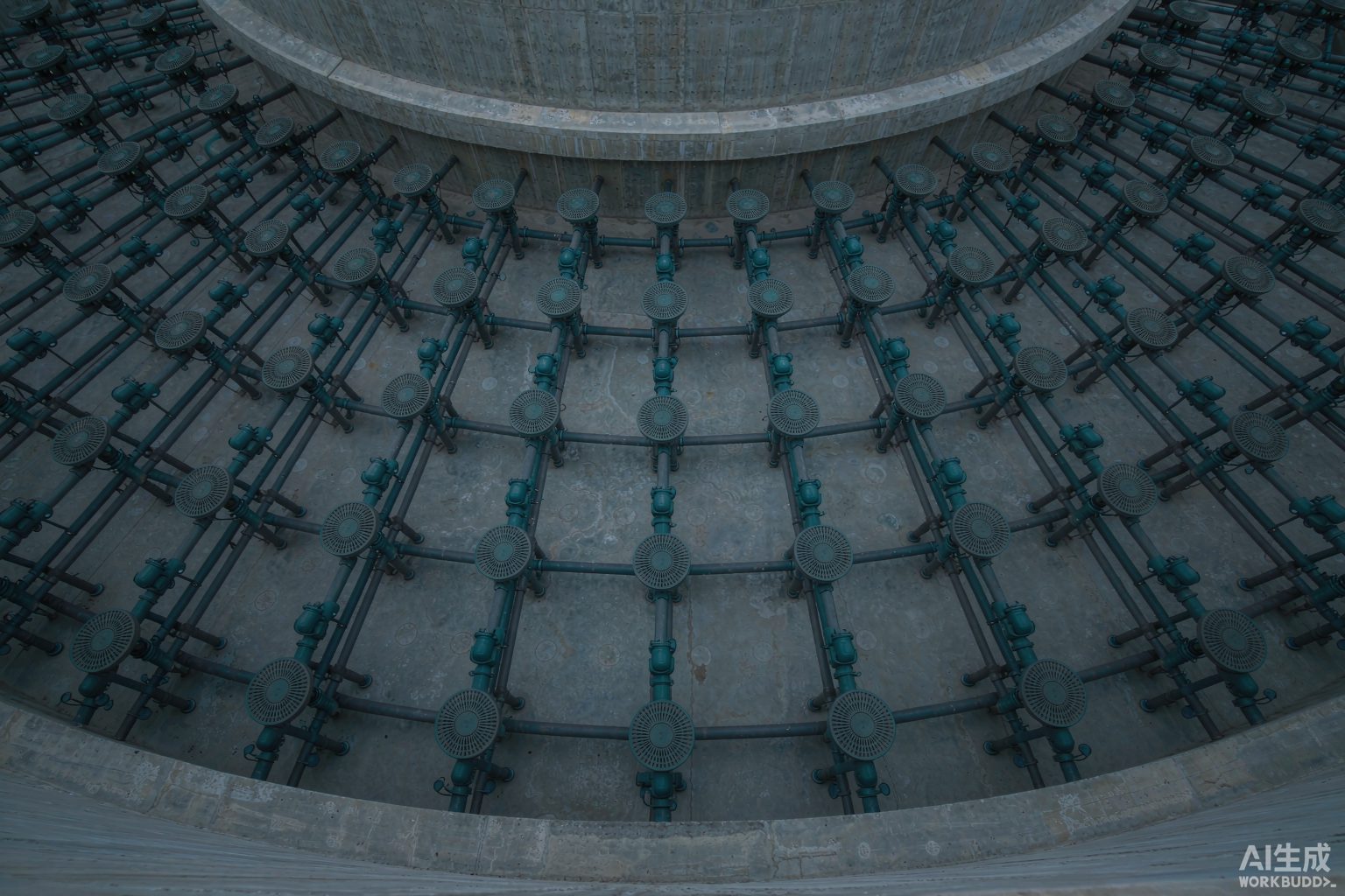
Method 1 (air flow rate method): first calculate the total aeration air flow rate for the whole tank, then divide by the reasonable air flow rate per aerator;
Method 2 (service area method): use the tank area of the aeration zone and divide by the service area per aerator.
And the manufacturer's recommendation is: if the two results are inconsistent, adjust the fan air flow rate, number of aerators, type, air flow rate per unit, and oxygen transfer efficiency within the parameter range, ultimately making N1 and N2 converge to the same number. Please note the meaning of this statement—it is not "the two methods validate each other," but "the two methods themselves give you a feasible region, and you have to pick a point within it."
| Method | Formula | Parameter range per unit |
|---|---|---|
| Method 1: Airflow method | N1 = Total design air volume of the tank ÷ Reasonable airflow per unit | Airflow 1.5~3.0 m³/(h·unit) |
| Method 2: Service area method | N2 = Aeration zone area ÷ Service area per unit | Service area 0.25~0.55 m²/unit |
| Another set of industry empirical criteria | Direct estimation by area | φ215 approx. 3 units/m²; φ260 approx. 2 units/m²; φ300 approx. 1.5 units/m² |
| High-concentration conditions | Densified according to oxygen demand | COD > 800 mg/L can be densified to 4~5 units/m² |
Substituting the ranges into the calculation immediately reveals the problem. [Self-calculation] Let the aeration zone area be 1000 m² and the design air volume be 5000 m³/h, using φ215:
· Service area method: 1000 ÷ 0.55 ≈ 1818 units (using the lower-limit area) to 1000 ÷ 0.25 = 4000 units (using the upper-limit area), a 2.2-fold difference between the two ends;
· Airflow method: 5000 ÷ 3.0 ≈ 1667 units to 5000 ÷ 1.5 ≈ 3333 units, a 2-fold difference between the two ends.
In other words, merely by choosing which point within the parameter range to use, the number of aerators in the same tank can vary between 1667 and 4000 units. What truly locks the two calculation methods together is a convergence point that falls within both ranges simultaneously: for example, taking 2500 units gives a per-unit service area = 1000÷2500 = 0.40 m² (falling within 0.25~0.55 ✔), and a per-unit airflow = 5000÷2500 = 2.0 m³/(h·unit) (falling within 1.5~3.0 ✔). This point exists, but the window is very narrow—which is why aerator selection cannot rely on a single calculated number, nor on a single "recommended quantity" quoted by a manufacturer.
IX. A single aerator has an "economic airflow window"—too small or too large is both wrong
The core evidence in this section comes from a real bench-scale comparison. The Frankenmuth wastewater treatment plant in Michigan, USA, converted coarse-bubble aeration to fine-bubble aeration in 1986 年, and its operating records contain a set of very telling figures: when the per-aerator airflow was 1 scfm, the actual oxygen transfer efficiency converted to aSOTE was 16.9%; when the airflow was doubled to 2 scfm, aSOTE dropped to 11.0%. With the same equipment and the same membrane diffuser, merely because the "airflow allocated per unit" doubled, efficiency fell by about 35%.
This is exactly why the "service area/airflow parameter range" must be selected with efficiency as the premise: spreading the airflow over more aerators (reducing per-unit airflow) can improve efficiency; but too low a per-unit airflow will cause clogging and worsen the stress on the piping network during low-load periods. In engineering practice, this window is roughly:
· For φ215 disc-type, the economic airflow range is about 1.5~2.5 m³/(h·unit) (product nominal range 1.5~3.0, and on site it should preferably fall in the lower part);
· For tubular aerators, the recommended airflow per tube is about 2~8 m³/(h·tube); exceeding this will cause a sharp increase in pressure loss or bubble coalescence;
· There is an upper-limit criterion for airflow per unit tank area: when the airflow per square meter of tank area exceeds 10 m³/h, bubble collision and coalescence begin to intensify, and oxygen transfer efficiency drops rather than rises;
· The plant-wide design air-to-water ratio is usually between 5∶1~15∶1, depending on influent concentration and treatment requirements.
[Self-check] Recheck with the convergence point above: 2500 units × 2.0 m³/h = 5000 m³/h, divided by the tank area 1000 m² gives 5 m³/(h·m²), which still has margin from the critical value of 10 m³/h.But if laid out as "densified to 4 units/m², 3.0 m³/h per unit", it becomes 12 m³/(h·m²), which has crossed the critical line—this is where the rule of thumb "high-concentration wastewater should be densified" most easily fails under shallow-tank, high-airflow conditions. If the "false boiling" phenomenon occurs on site—violent surface churning without a rise in dissolved oxygen—it often means the critical gas velocity has already been exceeded, and increasing airflow at that point only wastes electricity.
There is another nearly zero-cost source of failure: uneven air distribution. When the front end of the same branch pipe discharges more air and the end discharges less, the actual effective aeration area may be only 70%~80% of the design value; if the installation levelness deviation of the aerator exceeds 2 cm, it will cause different local water depths, resulting in "excessive aeration in shallow water zones and insufficient oxygen supply in deep water zones." For old retrofit projects, uneven tank bottoms are very common, and the cost is of the same order of magnitude as scaling.
X. How to Judge on Site That It Has Failed: Five Signals and Their Respective Thresholds
Membrane fouling is not a sudden event; it leaves five simultaneously appearing traces in instrument and blower trends. The key criterion is "same direction, lasting two months"—a single week of high Dissolved Oxygen is not a reason for cleaning, and the increase in Mixed Liquor viscosity in winter itself will lower α and raise the air volume demand.
| Signal | Symptom | Common Threshold |
|---|---|---|
| ① Airflow rises under the same load | More air is required to maintain the same DO setpoint | Airflow keeps rising under the same influent load |
| ② DO at the outlet drops | Residual DO at the tank outlet falls below target | Below 1.5–2.0 mg/L |
| ③ Blower back pressure rises | Outlet pressure rises year by year at the same airflow | Schedule cleaning when it rises by 50–100 m bar |
| ④ Annual power consumption climbs | kWh keeps rising while MLSS and F/M remain stable | 12-month rolling average rises by 5%–10% |
| ⑤ Insufficient peak airflow | Blowers are at their capacity limit yet DO still cannot be reached | Means the blower capacity limit has been reached |
On the equipment side, there are two more direct criteria: first, membrane differential pressure—a new membrane typically reads 0.02–0.04 MPa; when the differential pressure exceeds 0.08 MPa, replacement should be planned even if the appearance is intact; second, the efficiency decay threshold—public data give two replacement trigger lines: "oxygen transfer efficiency drop of more than 15%" and "drop of more than 20%". The 5 percentage point difference between the two thresholds is not a contradiction, but an engineering practice value under different membrane materials and different accounting bases. In practice, it is recommended to distinguish by "whether it can recover after cleaning": clean first if cleaning restores performance; replace only if it does not recover after cleaning.
XI. How Much Can Cleaning and Replacement Recover: Four Real "Recovery" Ledgers
| Project/Scale | Problem | Result |
|---|---|---|
| A major UK water utility (fine-bubble aeration system) | Membrane fouling and scaling, high blower backpressure, increased energy consumption | After online acid cleaning without shutdown: air flow increased by 65%, recovering 97% of original performance; at the same power, air delivery approximately 2 times that before cleaning |
| A 12 万 m³/d municipal wastewater treatment plant in East Asia (two-phase retrofit) | Phase I: tubular diffuser membrane pore fouling and bubble coalescence; Phase II: disc membrane stress cracking | Replaced with 10 608 φ270 EPDM disc diffusers; Phase I backpressure 76 kPa (design upper limit 81 kPa), Phase II 57.3 kPa (upper limit 61 kPa); after retrofit, aeration energy consumption reduced by approximately 48% |
| A 10 万 m³/d municipal wastewater treatment plant in East Asia | Aeration accounts for over 55% of operating costs; total system resistance rose to 76 kPa; Dissolved Oxygen (DO) fluctuation ±1.2 mg/L | Airflow reconfiguration + online acid cleaning; energy consumption reduced by 43%~49%, DO fluctuation narrowed to ±0.3 mg/L, payback period ≤1.5 年, annual carbon reduction approximately 450 t |
| Ridgewood Wastewater Treatment Plant, New Jersey, USA | Performance maintenance after 1983 年 fine-bubble retrofit | The 28% energy reduction is maintained through routine cleaning (EPA 832-F-99-065) |
| Frankenmuth Wastewater Treatment Plant, Michigan, USA | 1986 年 coarse-bubble to fine-bubble conversion; influent contains brewery wastewater at approximately 25%~30% flow and 50%~70% BOD load | Gas-phase cleaning scheduled when DWP reaches 16~18 in w.g.; no correlation established between cleaning and OTE—indicating that "cleaning" restores resistance, not necessarily mass transfer |
| A 10 万 m³/d municipal wastewater treatment plant in East China (blower side) | 4 220 kW Roots blowers, annual electricity cost approximately 620 万 yuan | Replaced with 3 160 kW air suspension blowers + constant-pressure variable air volume; pipe network operating pressure point 0.65→0.52 bar; aeration power consumption per ton of water 0.35→0.21 kWh, annual electricity savings approximately 196 万 kWh, payback period approximately 1.8 年 |
| A 5 万 m³/d industrial park wastewater treatment plant in East China | 3 Roots blowers | Replaced with 2 air suspension blowers (one duty, one standby); annual electricity consumption 186 万→139 万 kWh, annual savings approximately 32 万 yuan |
| A 5 万 m³/d wastewater treatment plant (integrated precision aeration solution) | Extensive aeration, excessive oxygen supply, carbon source supplementation required | Investment approximately 280 万 yuan (magnetic levitation blowers + variable-orifice diffusers + sensors + control platform); annual savings of approximately 32.85 万 yuan in electricity and 24 万 yuan in chemicals; comprehensive payback period approximately 4.1 年 |
The row most worth pausing on in this table is row 5 (Frankenmuth): cleaning effectively controlled DWP but failed to establish a correlation with oxygen transfer efficiency. It reminds us that "backpressure came down" and "mass transfer recovered" are two different things—backpressure governs blower electricity, while mass transfer governs basin oxygen. Both indicators must be examined during diagnosis; one cannot substitute for the other.
XII. The Blower Side: Specific Power, Noise and Maintenance Costs
The electricity cost of aeration is jointly determined by "air volume × pressure ÷ efficiency." Replacing only the aerators without replacing the blowers often captures only part of the benefit. A comparison of three common types of blowers is roughly as follows:
| Type | Specific Power kW/(m³/min) | Noise dB | Annual Maintenance Cost |
|---|---|---|---|
| Roots Blower | 4.2 | 105 | Approx. 8.2 万 CNY |
| Multistage Centrifugal Blower | 3.6 | 92 | Approx. 4.5 万 CNY |
| Magnetic Bearing / Air Bearing Centrifugal Blower | 2.9 | 78 | Approx. 0.3 万 CNY (mainly filter media replacement) |
Two characteristics that are easily overlooked but directly determine the return on investment: the first is the ability to maintain efficiency in the low-load range—conventional blowers experience a sharp drop in efficiency when airflow demand falls to 60%, whereas bearing-type blowers can still maintain relatively high efficiency, which means additional 8%~12% power savings for municipal plants with pronounced nighttime influent troughs; the second is the difference in speed control methods—switching from "fixed-frequency operation + valve throttling" to variable-speed regulation is a cheaper step than replacing equipment, and is often implemented first. The publicly accepted industry view is that a properly designed aeration control system alone can deliver a 25%~40% reduction in aeration energy consumption (related conclusions from US EPA), and this benefit is independent of equipment brand.
In addition, there is a compliance aspect: the noise from the blowers must comply with the "Emission Standard of Environment Noise for Boundary of Industrial Enterprises," and the operating noise should preferably be below 85 d dB(A). The gap between the Roots blower at 105 d dB and the levitation blower at 78 d dB often directly determines whether additional sound insulation is needed in the blower room.
XIII. Membrane Lifespan: The Same EPDM, Four Claims Differing by Up to Four Times
The membrane is a consumable, and its lifespan is the most error-prone item in selection calculations. Publicly available information gives conflicting figures for the expected lifespan of the same material—this is not because manufacturers are deliberately vague, but because the term "lifespan" itself has no unified definition (Is it the material failure lifespan, or the lifespan before efficiency falls short? Is it under municipal conditions or high-salinity conditions?).
| Material | Service-life metric 1 | Service-life metric 2 | Service-life metric 3 |
|---|---|---|---|
| EPDM (Ethylene Propylene Diene Monomer) | 2~4 年 (some procurement documents) | 3~5 年 (equipment technical documents) | 5~8 年 (English technical documents) |
| Silicone Rubber | 3~5 年 | 5~8 年 | 8~10 年 |
| Polyurethane (PU) | 1~2 年 | 2~4 年 | — |
| PTFE coating / PVDF fluororubber | 4~6 年 (PTFE coating) | 10 年 or more (PTFE coating) | 2~3.5 年 (PVDF/fluororubber, severe corrosive conditions) |
The root cause of the differences lies in the operating conditions rather than the material itself. The condition corrections given in the same document are highly informative: high-quality EPDM in light industrial wastewater (food, beverage, grain and oil) can last 3.5~5 年 before replacement; in medium-to-high oil/grease or high suspended solids wastewater (slaughterhouse, printing and dyeing, papermaking) it drops to 2~3 年; under high salinity and fluctuating acid/alkali conditions it drops to 1.5~2 年; while inferior recycled EPDM under harsh industrial conditions lasts only 6 months to 1 年 before hardening, cracking and clogging the pores. Two sets of extreme values can quantify this: in printing and dyeing wastewater with oil content exceeding 50 mg/L, ordinary EPDM shows significant performance degradation after about 6 months; in coastal petrochemical parks where chloride ions remain above 3000 mg/L year-round, ordinary EPDM may become brittle and crack within 6 months.
XIV. Engineering Truths
1. Catalog values are "admission values," not "design values." Writing "clean water 3.2 m water depth, SOTE ≥22%, power efficiency ≥4.5 kgO₂/kWh" in the procurement specification is a reasonable admission threshold, but substituting it directly into the air volume calculation as a design condition is equivalent to assuming your tank is a clean water tank.
2. When saying "discounted by 0.8," please specify which type of water it applies to. For domestic sewage, a discount of 0.7~0.8 is still debatable; for industrial wastewater containing oil and high concentrations of surfactants, 0.4~0.5 is the norm. This number is the most expensive assumption in the entire aeration sizing process.
3. The number of aerators must converge through two paths. Calculating only by the air flow method or only by the service area method will both yield a quantity that "looks right but does not fall into the parameter range." A convergence point exists, but the window is narrow — this is why manufacturers' parameter tables give ranges rather than points.
4. The low-load period is the most dangerous time for the aeration system. At this time it is not about "saving electricity"; rather, excessively low air flow leads to insufficient output per unit, only the top of the pipe receiving air, and worsened stress on membranes and pipe fittings, making failures more likely.
5. "Backpressure dropped" does not equal "mass transfer improved." What cleaning can restore is resistance; whether mass transfer can be restored requires looking at the relationship curve between dissolved oxygen and air flow. The two indicators correspond to electricity costs and effluent quality respectively, and cannot substitute for each other.
6. Get the control right first, then consider changing equipment. If the two practices of single-point dissolved oxygen setpoint and fixed-frequency operation plus valve throttling are not changed, switching to any type of high-efficiency equipment will only capture part of the benefits.
References
- Code for Design of Outdoor Wastewater Engineering GB 50014—2006 (2016 年 edition), Section 6.8 Oxygen Supply Facilities and clause explanations (including the explanation in Clause 6.8.3 that "the oxygen transfer performance of diffusers is the value under standard conditions (0.1 MPa, 20℃ clean water)").
- Ministry of Ecology and Environment, Technical Requirement for Environmental Protection Product: Medium and Fine Bubble Diffusers HJ/T 252—2006 (replacing HCRJ 031—1998), implemented on 2006-06-01.
- Determination of Clean Water Oxygen Mass Transfer Performance of Fine Bubble Diffusers CJ/T 475—2015 (executive standard for tubular fine bubble diffusers, including technical indicators such as design air flow rate, service area, and head loss).
- SUEZ Water Handbook, Aeration systems (aeration systems: definitions of SOTR/SOTE/SSOTE/SAE, clean water testing and correction factors Tp (α)/Td/Tt, mass of oxygen in air 0.3 kg/Nm³).
- US EPA 832-F-99-065 (1999), Wastewater Technology Fact Sheet: Fine Bubble Aeration.
- US EPA 600/R-94/100, Fine Pore Diffuser Case History for Frankenmuth, Michigan (1986—1988 operating records, 1 scfm and 2 scfm corresponding to aSOTE 16.9% and 11.0%, DWP 16~18 in w.g. cleaning trigger).
- Xylem technical documentation (2019—2022) and Diffuser Liquid Cleaning case report (a large UK water utility: air flow increased by 65%, original performance restored by 97%).
- HydropureWater, Diffuser Cleaning for Aeration Tanks: Engineering Guide (five field signals and thresholds of fouling: terminal DO 1.5~2.0 mg/L, backpressure rise 50~100 mbar, annual kWh climb 5%~10%).
- American Aeration, How Fine Bubble Diffusers Improve Oxygen Transfer (SOTE 2.0%~4.0 %/m; α for fine pores 0.4~0.7, coarse pores 0.65~0.9; Type I inorganic scaling and Type II biofilm; bubble coalescence).
- Water & Wastewater, Diffused Aeration (Field OTE ≈ SOTE×α×F; α for fine pores 0.4~0.65 versus coarse pores 0.6~0.85; F 0.6~0.9; worked example 3000 kgO₂/d, 26%/11% clean water SOTE, specific power 0.022 kW/(m³/h)).
- Studio Matrx, Aeration Design Principles for STPs and Wastewater Aeration Systems (α 0.4~0.8 for fine pores, β 0.90~0.98, F 0.8~0.9; SOTE 5~7 %/m, deep tank overall 25%~40%; measured case with field α≈0.46).
- NIHAOWATER, Energy Audit for Aeration Systems (four indicators SOTR/SOTE/OTR/SAE; SAE benchmark table: fine pore optimized 2.5~5.0, fine pore typical 1.8~3.5, coarse pore 1.2~2.0, low-speed surface aeration 1.2~2.5, high-speed surface aeration 0.8~1.5, jet aeration 1.0~2.0, deep well 3.5~6.0 kgO₂/kWh; θ=1.024).
- Study on the Influence of Membrane Pore Parameters and Surfactants on the Oxygen Transfer Performance of Fine Bubble Diffusers (abstract: aeration system energy consumption accounts for about 45%~75% of wastewater treatment plant energy consumption; SOTE decreases with increasing air flow rate, membrane pore spacing, and membrane pore diameter; correction factor α increases with increasing membrane pore diameter).
- Pilot study conclusions by Luo Tao et al. on the effect of sodium dodecylbenzene sulfonate (SDBS) on oxygen mass transfer in fine bubble aeration (within the SDBS range of 0~20 mg/L, KLa first decreases and then increases, cited via review literature).
- Existing research conclusions by Zhuang Jian et al. and Yu Jiangzhong et al. on the influence of pore diameter and aeration intensity on oxygen transfer performance (cited via review literature).
- AquaSust, Fine Bubble Disc Diffuser Upgrade Cuts Aeration Energy by 48% at 120,000 m³/d WWTP (Phase I tubular 2 248 units@8 Nm³/h, backpressure 76 kPa; Phase II disc 3 722 units, backpressure 57.3 kPa; replacement with 10 608 units φ270 EPDM; φ270 SOTE ≥30%, theoretical power efficiency ≥4.5 kgO₂/kWh, resistance ≤3.5 kPa).
- AquaSust, Aeration System Energy Optimization for a 100,000 m³/d Municipal WWTP (aeration accounts for more than 55% of operating costs; total system resistance 76 kPa; dissolved oxygen fluctuation ±1.2 mg/L→±0.3 mg/L; energy consumption reduced by 43%~49%; payback period ≤1.5 年; annual carbon reduction about 450 t).
- Public sample parameters of domestic disc fine bubble diffusers (φ215/φ260/φ300; service area 0.25~0.55 and 0.35~0.75 m²/unit; average operating pore size of membrane 80~100 μm; air flow rate 1.5~3 m³/(h·unit); oxygen utilization rate at water depth 3.2 m 18.4%~27.7%; power efficiency 4.46~5.19 kgO₂/kWh; aeration resistance 180~280 mmH₂O; installation height 270/250/200 mm).
- Domestic technical documentation for fine bubble diffuser selection (two methods for calculating the number of diffusers: air flow rate method N1 and service area method N2, which must converge; φ215 about 3 units/m², φ260 about 2 units/m², φ300 about 1.5 units/m²; insufficient air flow during low-load periods causes uneven stress on air pipes, making them prone to rupture).
- Domestic diffuser technical documentation (clean water 3.2 m SOTE 18%~28%, 6 m clean water SOTE 30%~38%, power efficiency 7~8.5 kgO₂/kWh; oxygen utilization rate increases by about 1 m~4 percentage points for every 6 increase in water depth; oxygen utilization rate decays by 2~3 年 after 20%~40% of membrane scaling during operation; efficiency discounted by 70%~80% under actual wastewater conditions; procurement tender thresholds SOTE ≥22%, power efficiency ≥4.5 kgO₂/kWh).
- Domestic procurement and technical encyclopedia documentation (when the air volume per square meter of tank area exceeds 10 m³/h, bubble coalescence intensifies and efficiency decreases instead of increasing; design air-water ratio 5∶1~15∶1; uneven air distribution makes the effective aeration area only 70%~80% of the design value; installation levelness deviation exceeding 2 cm causes over-aeration in shallow water zones and insufficient oxygen supply in deep water zones; optimal tank depth 4~6 m, efficiency increase slows down beyond 6 m).
- Domestic membrane technology and procurement documentation (service life and working condition correspondence of EPDM/silicone rubber/polyurethane/PTFE coating/PVDF; membrane differential pressure 0.02~0.04 MPa for new membranes, planned replacement required when exceeding 0.08 MPa; when hardness exceeds 300 mg/L, micropores may partially close within 6 months; international brands 400~600 元/unit, domestic brands 200~350 元/unit; 300 万 open-close cycle test; two replacement thresholds of efficiency drop 15% or 20%).
- Domestic blower technical documentation (specific power under the same working conditions: Roots 4.2, multistage centrifugal 3.6, magnetic levitation 2.9 kW/(m³/min); noise 105/92/78 dB; annual maintenance cost 8.2/4.5/0.3 万 yuan; maintaining high efficiency at low load and additional power savings of 8%~12%; motor efficiency and noise compliance requirements).
- Domestic wastewater treatment plant retrofit case reports (a certain 10 万 m³/d plant in East China: 4×220 kW Roots→3×160 kW air suspension, pressure point 0.65→0.52 bar, aeration power consumption per ton of water 0.35→0.21 kWh, annual power savings of about 196 万 kWh, payback period about 1.8 年; a certain 5 万 m³/d industrial park plant in East China, annual power consumption 186 万→139 万 kWh).
- Public materials on domestic integrated precision aeration solutions (a certain 5 万 m³/d plant invested about 280 万 yuan, annual electricity cost savings of about 32.85 万 yuan and chemicals savings of about 24 万 yuan, comprehensive payback period about 4.1 年; including the cited EPA conclusion that "the aeration control system itself can reduce energy consumption by 25%~40%").
Note: All data in this article are annotated with the nature of their sources. Equipment sample parameters, manufacturer cases, and third-party testing data have been separately noted when cited. Before using them for design or price comparison, readers are advised to verify against the original standard texts and test reports.
您提供的内容似乎不完整,缺少需要翻译的中文文本。请提供待翻译的中文内容,我将根据术语表为您翻译成地道的英文。