



 Multi-industry nationwide coverage (chemical wastewater in industrial parks, pri
 Pilot to full-scale engineering (0.35 to 120,000 m³/d; membrane area per plant 6
Membrane Module Selection: There Are Six Flux Values, but Only 15~20 Is Usable
A membrane sample, three engineering standards, and a plant that has been running for over a decade yield three mutually unequal numbers; and the intersection of these three standards leaves only a narrow band.
The most common mistake in membrane module selection is treating the flux on the first page of the manufacturer's sample as the design flux. That number is the factory inspection value for pure water, 10 kPa, new membrane, 25℃; the upper limit given by the standard is 120~750 L/(m²·h); while the actual operating flux permitted to be written into the design document, the ranges given by the three current standards are 10~20, 12~30, 15~25 respectively, with an intersection of only 15~20 L/(m²·h). The two differ by a factor of 4 to 25. This article breaks down the four most error-prone bases: flux, the denominator of membrane area, differential pressure threshold, and integrity criterion.
I. The number on the sample is a factory inspection value, not a design parameter
HJ 2010—2011 "Technical Specification for Membrane Bioreactor Wastewater Treatment Engineering" Article 7.1.2 lists the "principles to be followed in selecting membrane modules," the first of which is pure water flux 120 L/(m²·h)~750 L/(m²·h), with 10 kPa noted in parentheses. The immediately following Article 7.1.3 is the design operating flux: hollow fiber membranes take 12~30, flat sheet membranes take 16~50. In the same standard, two adjacent articles, the numbers differ by a factor of 4 to 25.
This is not a contradiction in the standard; the two articles answer two different questions. 7.1.2 answers "whether this membrane itself passes water," measured with pure water, excluding sludge, excluding concentration polarization, excluding fouling, measuring the hydraulic resistance of the membrane material; 7.1.3 answers "how much water it can still stably produce after soaking in sludge mixed liquor for three years," measuring the entire system. The former is a factory inspection value, the latter is the design parameter.
Putting these two numbers in, and superimposing the measured values of three real projects, the flux of a single membrane has six mutually unequal numbers (Table 1).
| Name | Value | Reference Conditions | Source |
|---|---|---|---|
| Pure Water Flux | 120~750 | Pure water, 10 kPa, new membrane | HJ 2010—2011 Clause 7.1.2 a) |
| Design Operating Flux (Submerged · Hollow Fiber) | 12~30 | Sludge mixed liquor, design water temperature | Ibid. Clause 7.1.3 |
| Design Operating Flux (Submerged · Flat Sheet) | 16~50 | Ibid. | Ibid. Clause 7.1.3 |
| External (Cross-Flow) Flux | 40~150 | Membrane surface velocity 3~5 m/s, 0.2~0.4 MPa | Ibid. Clause 6.3.3.7 d) |
| Measured at 19 10,000-ton-scale plants | 15~25, median 19.6 | Actual operation, full year | The MBR Site survey |
| Measured at Miyun 4.5 万 m³/d | Instantaneous 32.3 / Net 28.3 | Average TMP 18.2 kPa, weekly online cleaning | Yu Kaichang, Huang Xia (2008) |
The two measured values in the last column of Table 1 deserve a closer look. The difference between the instantaneous flux 32.3 and the net flux 28.3 at Miyun is 4.0, accounting for 12.4%—this 12.4% is not a membrane problem, but rather "there are periods of the day when no water is being produced at all." This difference is discussed separately below.
A standard number that needs clarification. A large amount of second-hand online material (including some manufacturers' selection manuals) states that "HJ 579—2010 'Technical Specification for Wastewater Treatment Engineering by Membrane Bioreactor Process' specifies a design flux of 12~30 L/(m²·h)". This statement is wrong in two places. First, the actual title of HJ 579—2010 is 'Technical Specification for Wastewater Treatment Engineering by Membrane Separation Process'; its scope of application states that the membrane separation processes referred to are microfiltration, ultrafiltration, nanofiltration and reverse osmosis, and explicitly states that it "does not apply to membrane separation engineering for wastewater treatment and reuse using the membrane bioreactor process and charged membranes". Second, it is HJ 2010—2011 'Technical Specification for Wastewater Treatment Engineering by Membrane Biological Process' that specifies 12~30. Both the standard number and the scope of application are mismatched, while the numbers happen to be correct—this type of error is the hardest to detect, because it withstands the test of "checking that 12~30 does indeed exist".
II. Three standards, three ranges, with an intersection of only 15~20
What is more troublesome is that even if the standard number is cited correctly, the range is not unique. In the current system, at least three engineering construction standards govern the membrane flux of MBR, and the values they give are not the same (Table 2).
| Standard | Hollow Fiber Membrane | Flat Sheet Membrane | Tubular Membrane | Remarks |
|---|---|---|---|---|
| HJ 2010—2011 Membrane Biological Process | 12~30 | 16~50 | — (External 40~150) | Environmental protection industry engineering specification |
| GB 50014—2021 Standard for Design of Outdoor Wastewater Engineering | Submerged 15~25 (configuration not distinguished) | External 30~45 | Article 7.6.44 | |
| Technical Standard for Wastewater Treatment Engineering of Medical Institutions | 10~20 | 12~25 | 25~50 | Article 7.2.16 (draft for comments) |
| Intersection of the three (hollow fiber) | 15~20 | |||
The values in the three standards each have their own rationale: HJ 2010 follows the environmental protection perspective, governing whether "this facility can stably meet the discharge standards," so its values are relatively broad; GB 50014 follows the water supply and drainage design perspective, and Article 7.6.43 additionally requires that "the operating flux of the membrane system shall be less than the critical flux," and checks the peak flux and forced flux based on the design flow of the biological reaction tank, so its values are conservative; the standard for medical institutions addresses small-scale facilities with large water quality fluctuations and weak operation and maintenance capabilities, so its values are even more conservative.
For designers, the conclusion is very practical: when three standards apply simultaneously and you do not want to be questioned about the basis during review, setting the design flux of hollow fiber membranes within 15~20 is the least troublesome approach. This range satisfies all three standards at the same time, and therefore also satisfies three sets of review logic.
By the way, GB 50014—2021 Clause 7.6.45: when laying out membrane modules, reserve 10%~20% of spare membrane module positions as standby. This clause is easier to overlook than the flux value, because it governs the tank, not the membrane. As will be seen in Section 3 below, this clause and the membrane area calculation are two separate matters, and missing either one will incur costs on site.
III. The denominator of the area is not 24 小时
The basic calculation method for membrane area is design flow divided by design flux—something even a primary school student can do. But the unit of flux is "per square meter per hour," and how many hours that "per hour" actually refers to determines whether the membrane area differs by 20% or 38%.
HJ 2010 Clause 7.1.6.2 a) explicitly requires: set the operating frequency of the membrane module, i.e., the on and off times of intermittent pump operation (the example given in the standard is permeate production for 9 min, stop for 1 min); the on/off ratio should be set through testing, and from this the actual daily operating hours of the membrane module are calculated. Immediately following, clause b) gives the calculation method for the suction pump flow rate: membrane system design flow ÷ actual daily operating hours × safety factor (1.2~1.5).
This clause is about the pump, but the same "actual operating hours" must be fed back into the membrane area. Because "9 on, 1 off" means water is produced for only 21.6 h per day, not 24 h. Let's calculate it using Table 3 with 10 000 m³/d, 20 L/(m²·h).
| Calculation Method | Hours in Denominator | Required Membrane Area (m²) | Relative to the First |
|---|---|---|---|
| Based on 24 h continuous permeate production | 24 | 20 833 | 1.00 |
| Based on permeate production 9 min / stop 1 min | 21.6 | 23 148 | 1.11 |
| Further deducting backwash and maintenance cleaning downtime | 20.0 | 25 000 | 1.20 |
| Plus 15% end-of-life flux decay margin | 20.0 | 28 750 | 1.38 |
The difference between 32.3 and 28.3 at Miyun is the measured version of the third calculation method: instantaneous flux is the flux at the moment of pumping, while net flux is the flux after apportioning the non-production time back. If the design document specifies instantaneous flux and uses 24 h when calculating the area, both are optimistic, and combined they result in an area shortfall of 12%~20%. The shortfall will not be exposed during acceptance; it will be exposed during the first summer's high-temperature, high-load period.
Here, two separate calculations must be kept apart:
- Membrane area is calculated based on net flux, i.e., the denominator uses the actual hours of water production, plus an end-of-cycle decay margin.
- Membrane tank volume and module positions shall follow GB 50014 Clause 7.6.45, with an additional clearance of 10%~20% reserved.
The former is "how much membrane to buy," the latter is "how much space to leave in the tank." A common mistake is to fill the tank completely with the calculated membrane area, leaving not a single gap. When the flux drops in the second year, the only option is to force the flux up—and once the flux exceeds the critical value, the transmembrane pressure begins to climb unidirectionally, and the cleaning cycle becomes progressively shorter.
IV. Temperature: the fifteenth power of 1.03
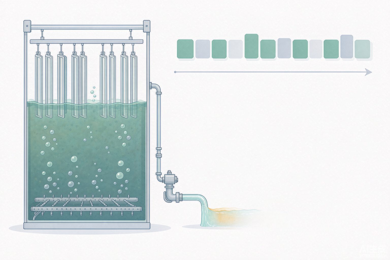
There is a widely used industry empirical formula for temperature correction of flux: TCF = 1.03^(25 − T), with 25℃ as the reference; for every 1℃ drop in water temperature, the membrane flux decreases by approximately 3%. This formula originally comes from Reverse Osmosis standardization practice, but the temperature effect on membrane flux has the same origin—water viscosity increases as temperature decreases, and membrane permeation resistance rises accordingly—so it has been widely borrowed for Ultrafiltration and MBR conversion.
| Water Temperature (℃) | TCF | 25℃ calibrated at 20 LMH, actual achievable (LMH) |
|---|---|---|
| 5 | 0.55 | 11.0 |
| 10 | 0.64 | 12.8 |
| 12 | 0.68 | 13.6 |
| 15 | 0.74 | 14.9 |
| 20 | 0.86 | 17.3 |
| 25 | 1.00 | 20.0 |
| 30 | 1.16 | 23.2 |
HJ 2010 Article 6.3.3.4 states: "The design water temperature of the biological reaction tank should be 12℃~38℃, and insulation or heating measures should be taken in winter in northern regions." Note that it governs the biological aspect—the activity of nitrifying bacteria decreases below 12℃, which is a biological constraint. The temperature effect on flux, however, is a physical constraint. Both happen to fall near 12℃, making them easy to mistake for the same thing.
The actual pitfall is here: manufacturers typically calibrate flux at 25℃, and design institutes often directly take the calibrated value and fill it into the 7.1.3 range during equipment selection. If this plant is in the north, with an actual winter water temperature of 10℃, then 20 LMH is left with only 12.8 LMH—just pressing right against the lower limit 12 of HJ 2010. In other words, the seemingly prudent approach of "taking the midpoint of the range" has actually already hit the lower limit during low-temperature months, leaving no margin at all for influent fluctuations. The 13.6 LMH in the 12℃ row of Table 4 illustrates the same point: if the design water temperature is not 25℃, then the statement "select according to 20 LMH" does not hold in winter.
The chain reaction that actually occurs in winter is clearly described in the survey of 19 ten-thousand-ton-scale plants: membrane permeability is generally lower in winter, and the measures taken on site are adjusting sludge discharge to control sludge concentration, increasing membrane scouring air flow, and increasing backwash frequency and online chemical cleaning frequency. All three measures add to operating costs, yet their cause is merely a flux that was not temperature-corrected.
V. Pressure Difference: Four Numbers—60, 50, 40, 20
Transmembrane pressure (TMP) is the only operating parameter of a membrane system that truly needs to be monitored every day, but it has four different thresholds, each belonging to a different matter (Table 5).
| Value | Meaning | Source |
|---|---|---|
| 0~60 kPa | Design transmembrane pressure difference range for hollow fiber membranes | HJ 2010 Table 2 |
| 0~20 kPa | Design transmembrane pressure difference range for flat sheet membranes | HJ 2010 Table 2 |
| 50 kPa | Maximum TMP (warranty boundary) given by most membrane manufacturers | The MBR Site survey |
| 40 kPa/50 kPa | Negative pressure 0.04 MPa alarm, 0.05 MPa suction pump auto-stop | HJ 2010 Clause 8.2.3.4 b) |
Two things need attention when reading this table. First, 60 and 20 differ by three times, and this difference has nothing to do with membrane material but with configuration: flat sheet membranes are supported by a frame, and when the pressure difference across the two sides is too large, the membrane plate will be pressed against the flow guide plate and the flow channel will be crushed shut; hollow fiber membranes are flexible, and no matter how large the pressure difference is, it only compresses the membrane fibers together, which is still mechanically tolerable. Therefore, when the configuration of the same tank is changed, the selection of the suction pump must be changed accordingly—a pump selected according to 60 kPa installed on a flat sheet membrane system will have more than half of its head unusable by the system, and using it will crush the membrane plates.
Second, the two numbers 40 and 50 are not design values but protection values. Their meaning is "when this point is reached, the automatic control system must act," not "designing to this point counts as acceptable." The true design values should be much lower: the measured TMP of 19 ten-thousand-ton-scale plants is 13~39 kPa, the long-term average at Miyun is 18.2 kPa, and at that industrial park in Shanghai, after replacing microfiltration membranes with ultrafiltration membranes, TMP remained stable below 10 kPa at an operating flux of 15~20 LMH.
The Shanghai case deserves separate discussion. It is a 5.0 万 m³/d industrial park wastewater plant with two treatment trains at one plant, of which the 2.5 万 m³/d chemical wastewater train originally used microfiltration membranes and was technically upgraded to ultrafiltration membranes. The water volume did not change, the tanks did not change, and the flux was not raised (15~20 LMH); only the membranes were replaced, yet TMP dropped from its normal level to below 10 kPa, aeration power consumption per ton of water fell by about 40%, and membrane cleaning costs fell by about 44%. These two percentages indicate the same thing: high pressure difference is not because the membrane is dirty, but because the flux was set in an unsustainable range. Cleaning can only push the pressure difference back down once; choosing the wrong flux will make it climb back again and again.
VI. Configuration: Inside-Out 1/6 and That 400
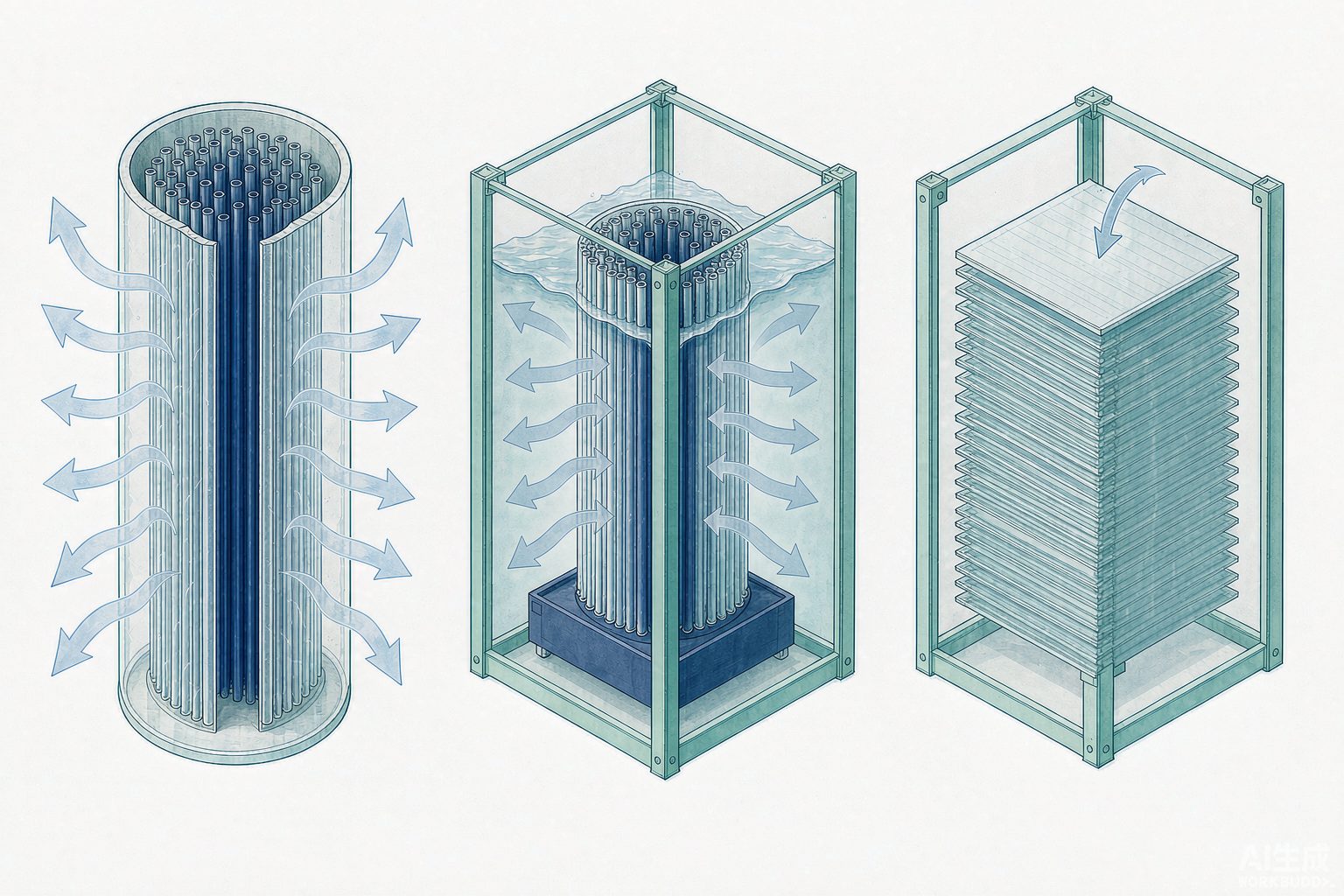
Hollow fiber membranes are divided into inside-out and outside-in types; the difference is not in the material but in the direction the water flows. In the inside-out type, raw water flows through the lumen of the membrane fibers and permeates from the inside out; in the outside-in type, raw water flows on the outside of the membrane fibers and permeates from the outside in. Once the direction is reversed, two engineering constraints emerge.
The first is particle size. In the inside-out type, the influent flow channel is the membrane fiber lumen; when the influent particle diameter is greater than 1/6 of the membrane fiber inner diameter, bridging and clogging may occur at the lumen inlet. This 1/6 is a very rigid criterion: common hollow fiber inner diameters are 0.7~1.3 mm, corresponding to a maximum allowable particle size of only 0.12~0.22 mm. That is to say, the inside-out type must have reliable pretreatment upstream, and usually also requires security filtration.
The second is concentration. This one is often overlooked, but it can be calculated. Assume influent suspended solids of 20 mg/L, cross-flow filtration, and a single-pass recovery rate of 95%; then the concentration factor = 1 ÷ (1 − 0.95) = 20 times, and the suspended solids concentration inside the membrane fiber near the outlet end = 20 × 20 = 400 mg/L. And that location happens to be where the flow velocity inside the tube is lowest. Low flow velocity plus high concentration means clogging occurs here, and it occurs inside the membrane fibers—physical flushing cannot reach it, and only chemically enhanced backwashing or offline cleaning can address it.
The outside-in type does not have this problem: the influent side is outside the membrane fibers, there is free space between the fibers, and the lumen always contains clean permeate. The cost is a slightly lower packing density, a slightly larger volume for the same permeate production, and more troublesome broken-fiber locating—broken fibers in the inside-out type can be checked one by one from the end seal and individually plugged, whereas this is much more difficult for the outside-in type. The comparison of the four configurations is shown in Table 6.
| Item | Hollow Fiber · Inside-Out | Hollow Fiber · Outside-In | Flat Sheet Membrane | Tubular Membrane |
|---|---|---|---|---|
| Packing Density | High | High | Medium | Low |
| Influent Suspended Solids Tolerance | Low (particles > 1/6 of inner diameter cause bridging) | Relatively High | Medium (wider flow channel) | High |
| Air Scouring Applicability | Not Recommended | Applicable (combined air and water) | Applicable (large-bubble scouring) | Not Suitable (relies on cross-flow velocity) |
| Broken Fiber Location and Single-Fiber Plugging | Relatively Easy (check at end seal) | Relatively Difficult | Single sheet can be replaced as a whole | — |
| Typical Flux (L/(m²·h)) | 12~30 | 12~30 | 16~50 | 40~150 (external configuration) |
| Application Scenarios | Surface water and clean water with adequate pretreatment | Wastewater reuse, large water quality fluctuations | Medium water volume, requires opening for inspection | High solids content, high-value materials |
VII. Integrity: No Turbidity Alarm Does Not Mean the Membrane Is Intact
Membrane module integrity testing falls into two categories: direct methods and indirect methods. These two categories do not answer the same question.
The indirect method involves installing a turbidimeter and a particle counter on the permeate pipe to continuously monitor effluent water quality. Its advantages are that it is continuous, automatic, and requires no shutdown; its disadvantage is insufficient sensitivity — if a small number of broken membrane fibers does not cause a sudden change in permeate water quality, the turbidimeter cannot identify or alarm it. The reason is simple: the bypass flow from a single broken fiber is an extremely small number relative to the total permeate flow, and is diluted by the large volume of qualified permeate.
The direct method is based on the bubble point principle: after fully wetting the membrane, compressed air at a pressure below the bubble point pressure is introduced on the permeate side; the liquid in intact membrane pores will not allow air to pass through noticeably under the action of surface tension; if defects or broken fibers exist, a large amount of air passes through the defects, and continuous bubbles can be seen when the other side is filled with liquid. There are two engineering approaches: the bubble observation method (immerse the module in water, adjust the pressure regulator to 1 bar, and observe whether continuous bubbling occurs; suitable for manual testing) and the pressure decay method (pressurize to 1 bar, close the inlet valve after stabilization, and measure the pressure drop rate; can be manual or automatic). The standard specifically notes: a single bubble that appears only after a very long time is a diffusional bubble and shall not be used as a basis for determining membrane fiber leakage.
The basis for testing frequency must likewise be clarified. Under U.S. drinking water regulatory practice, if a membrane system is to receive log removal credit, direct integrity testing is required once per day; wastewater MBR has no such mandatory requirement, and industry practice is generally once per week to once per month. The difference between the two is not diligence, but whether "the integrity of this membrane is treated as a compliance barrier." For industrial reuse projects, if the effluent is to enter Reverse Osmosis / RO or be directly reused in production, one should in practice hold oneself to the drinking water basis — because it is precisely the barrier function that it bears.
The real value of the pressure decay method is not "discovering a leak," but converting the leakage amount into a log removal value. The definition is LRV = log₁₀(permeate flow ÷ bypass flow). An LRV of 4 means the allowable bypass amount is one ten-thousandth of the permeate flow. Table 7 uses a publicly available calculation example to place two plants differing in scale by a factor of 34 side by side.
| Item | Large Plant | Small Plant |
|---|---|---|
| Permeate capacity | 120 000 m³/d | 3 500 m³/d |
| Membrane module configuration | 8 units × 396 elements × 14 500 membrane fibers | 96 elements × 14 500 membrane fibers |
| Total number of membrane fibers (calculated) | 4 594 万 fibers | 139 万 fibers |
| Allowable bypass at LRV 4 (calculated) | 12 m³/d | 0.35 m³/d |
| Maintenance interval to maintain LRV 4 | 6 months (allowable fiber breakage rate is 2 times the expected value) | More frequent intervention required |
| Maintenance interval to maintain LRV 4.5 | 3~4 months | — |
Three points should be drawn from this table.
Layer 1: LRV is a function of the maintenance cycle, not a water quality indicator. In the same plant, if 4 is required, intervention is needed once every six months; if 4.5 is required, intervention is needed once every three to four months. Therefore, the statement "our membrane effluent turbidity is 0.2 NTU" cannot answer the question "is the membrane intact?"—it only indicates that there is currently no leakage visible to the turbidimeter.
Layer 2: The allowable number of broken fibers scales down proportionally with plant size. A large plant allows 12 m³/d bypass, while a small plant allows only 0.35 m³/d, a difference of 34 times (120 000 ÷ 3 500 = 34.3), which exactly equals the size ratio. Since a single maintenance intervention addresses one or a few fibers, the same broken fiber consumes 34 times more margin in a small plant than in a large plant. This is why public materials explicitly state that "small-scale installations require higher intervention frequency."
Layer 3, which is also the layer most prone to calculation errors: broken fibers cause almost no loss of membrane area, yet completely compromise water quality. Based on a fiber outer diameter of 1.3 mm and an effective length of 2 m, the area of a single fiber = π × 0.0013 × 2 ≈ 0.008 m² (calculated independently). If 1 000 fibers break in a 1 500 m² module, the area loss is 8 m², accounting for 0.5%. Therefore, "broken fibers" can be ignored in the capacity account but cannot be ignored in the water quality account. The converse also holds: observing no significant change in permeate flow does not allow one to infer that the membrane is intact.
VIII. Air Scouring: SADp Reduced from 10 to 2
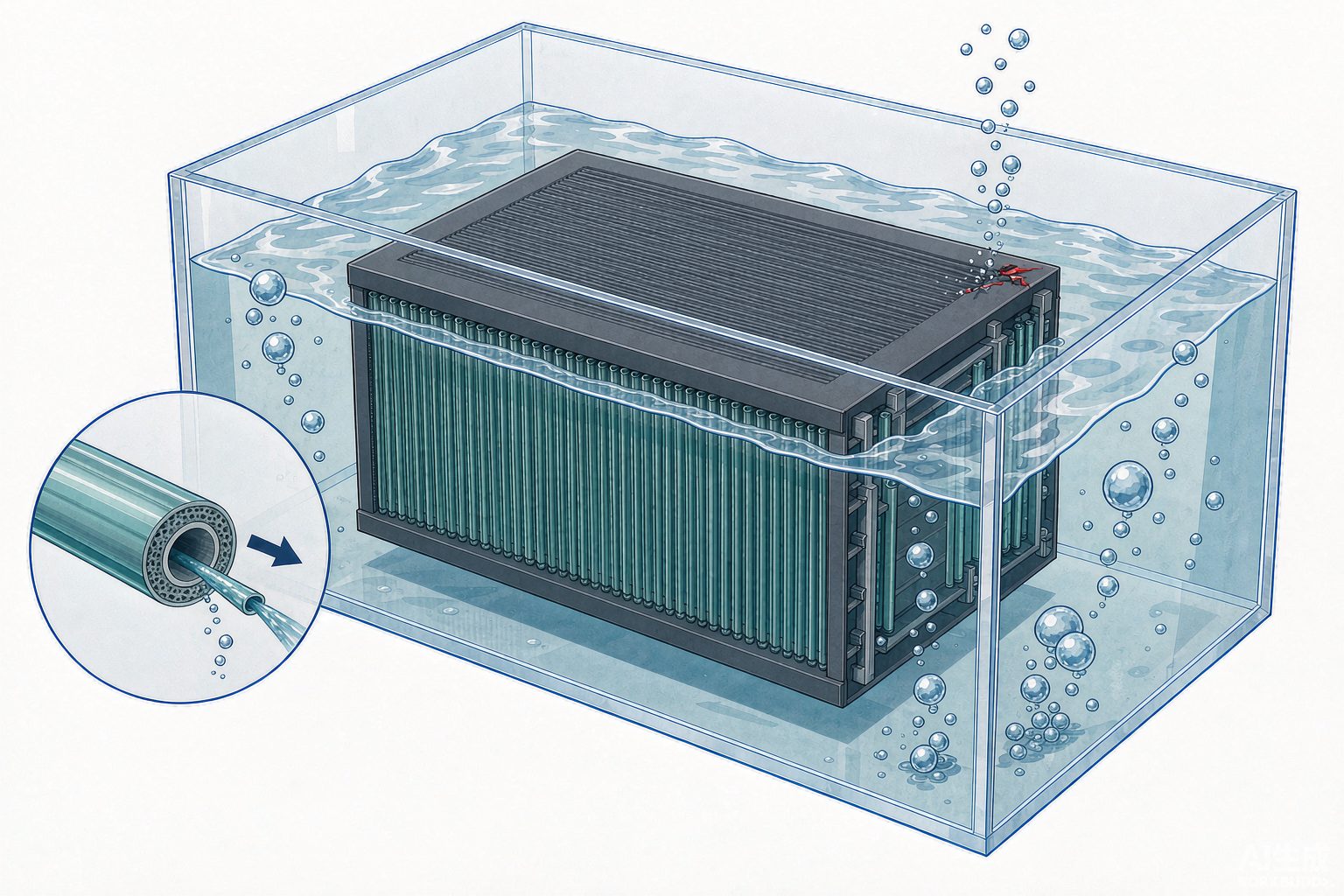
There is a dedicated metric for the power consumption of membrane systems: SADp, i.e., the amount of scouring air consumed per 1 m³ of water produced (Nm³/m³). It binds "air flow rate" and "permeate flow rate" into a single number, avoiding incomparable descriptions such as "the air flow is large but the water volume is also large."
| SADp (Nm³/m³) | Scouring power consumption (kWh/m³) | Remarks |
|---|---|---|
| 8~10 | 0.17~0.21 | Historically recognized value for fully optimized submerged MBR |
| 2 | 0.042 | A measured report value at 20 L MH |
| Reference: process aeration | 0.108 | Same report |
This table allows a clean back-calculation check: 0.042 ÷ 2 = 0.021, 0.17 ÷ 8 = 0.021, 0.21 ÷ 10 = 0.021. The three ratios are consistent, indicating that the implicit constant of "approximately 0.021 kWh per Nm³ of air" is self-consistent, and that SADp and scouring power consumption are indeed two expressions of the same number. Only after the check passes can it be used for comparison.
Following this number downward, one can understand why energy-saving discussions of membrane systems always revolve around aeration. Publicly available information is not entirely consistent regarding the proportions: some say membrane scouring aeration accounts for 34% of system energy consumption, biological aeration 42%, sludge return 10%, and pumps 4%; some say aeration scouring accounts for more than 80% of total system energy consumption; and there is also an estimate, self-noted by the author as "collected from the internet, for reference only," giving scouring aeration as 75% of membrane system power consumption, corresponding to 37.5%~42.5% of the whole plant when the membrane system accounts for 50% of plant power consumption. These differences in proportions arise from different denominators (membrane system/whole plant), different processes (whether denitrification is included), and whether biological aeration and membrane scouring aeration are metered separately. Before use, ask what the denominator is.
Once the air flow rate is reduced, there is another reverse pitfall: cleaning frequency and chemical concentration trade off against each other. Article 7.1.7.1 of HJ 2010 stipulates that for online cleaning frequency, hollow fiber membranes should be cleaned no less than once per month, flat sheet membranes may be cleaned once every 2~3 months, the chemical dosage is prepared at 2.0 L/(m²·time), and the concentration should be 1‰~3‰; offline cleaning is performed once every six months to one year at a concentration of 3‰~5‰. However, publicly available operating experience clearly states that when cleaning frequency is increased, the sodium hypochlorite solution needs to be adjusted to a lower concentration to maintain the same chemical dosing mass load.
A unit pitfall of an order of magnitude. The officially released version of HJ 2010 states that the online cleaning chemical concentration "should be 1‰~3‰", while the draft for comments of 2010 年 states "1%~3%". A difference of one per mille sign means a difference of ten times. Both formulations can be found in secondary sources, and both claim to come from HJ 2010. When citing this clause in selection or O&M documents, please verify against the released version; preparing the chemical at 1%~3% but using it at a frequency of 1‰~3‰ is equivalent to dosing ten times more available chlorine each time, and the oxidation resistance life of the membrane material will fail first.
IX. Key Parameter List
Divided into two tables: one governs selection and layout (determined once and for all), and the other governs operation and protection (needed every day). The reminder about the basis after each row is more error-prone than the numerical value itself.
| Parameter | Value / Range | Basis Reminder |
|---|---|---|
| Design operating flux (hollow fiber) | 15~20 L/(m²·h) | Intersection of three standards; correction required based on design water temperature |
| Design operating flux (flat sheet) | 16~25 L/(m²·h) | Conservative side of the intersection of three standards |
| Denominator for membrane area | Actual water production hours per day | Deduct shutdown for suction stop, backwash, and CEB |
| Spare slots for membrane modules | 10%~20% | GB 50014 Clause 7.6.45, governs tank not area |
| Membrane pore size | 0.01~0.4 μm | MF and UF in the same range; pore size cannot distinguish processes |
| Membrane life (design conditions) | Hollow fiber ≥3 年; flat sheet ≥5 年 | HJ 2010 Clause 7.1.1 |
| Membrane module layout spacing | From tank wall ≥300 mm, from water surface at top ≥400 mm, from tank bottom ≥300 mm | HJ 2010 Clause 7.1.5 |
| Parameter | Value / Range | Basis Reminder |
|---|---|---|
| MLSS (design) | Hollow fiber 6~12 g/L; flat sheet 6~20 g/L | HJ 2010 Table 2 |
| MLSS (operation control) | Hollow fiber 3~10 g/L; flat sheet 6~20 g/L | HJ 2010 Clause 8.2.2.1, not the same as design value |
| Transmembrane pressure (design range) | Hollow fiber 0~60 kPa; flat sheet 0~20 kPa | Determined by configuration, not material |
| Transmembrane pressure (protection action) | 0.04 MPa alarm / 0.05 MPa pump stop | HJ 2010 Clause 8.2.3.4 |
| Design water temperature | 12~38℃ | Biological constraint; flux also has physical temperature effects |
| Online cleaning | At least once per month; 2.0 L/(m²·time); concentration 1‰~3‰ | Note it is per mille, not percent |
X. Six Engineering Truths
- The high removal rate of MBR is not provided by the membrane. Article 6.1.6 of HJ 2010 requires the system to achieve removal rates for COD, BOD₅, SS, and ammonia nitrogen above 90%, 95%, 99%, and 90%, respectively. However, a pilot test at the Foshan Printing and Dyeing Industrial Park provided a set of controls: the average rejection rates of two types of flat-sheet membranes for biologically treated effluent were only 52.5% and 56.8% for COD, 67.8% and 64.1% for BOD₅, and 23.9% and 24.1% for Total Nitrogen / TN. The membrane retains suspended and colloidal matter, while dissolved COD passes through as before. In the system's 90%, the vast majority is the work done by the biological stage. These two percentages each have their own denominator and cannot be interchanged.
- Salt will suppress the flux. In a study of MBR for tannery wastewater in Taiwan, the on-site discharge water had a TDS of 8 700~9 700 mg/L (mainly chloride and sulfate), and the sustainable flux was only 4.92~8.17 L/(m²·h), far below the conventional 20~30. With the same membrane and the same tank, once the osmotic pressure and salinity change, the sustainable flux changes by orders of magnitude. Therefore, when selecting membranes for high-salinity wastewater, look at the salt first, then the membrane.
- Pure water flux is a factory inspection item, not a design parameter. It can only partially answer even the question of "whether this membrane is good," because the range of 120~750 is as wide as sixfold, and where it falls within this range depends more on the hydrophilic modification of the membrane material than on operational performance.
- "Leaving 10%~20% of space" and "adding 15% of area margin" are not the same money. The former is civil works, and the latter is equipment. Saving on civil works and maxing out equipment is equivalent to selling off future adjustment means in exchange for a one-time investment saving.
- Online cleaning concentration should be read in per mille. 1‰~3‰ and 1%~3% differ by a factor of ten, and this number determines the membrane's oxidation resistance life, not how obvious the cleaning effect is for that particular cleaning.
- Turbidity is an indirect indicator and is only responsible for its own sensitivity. An effluent of 0.2 NTU means "no leakage visible to the turbidity meter," not that the membrane is intact. To prove integrity, only direct method testing can be used, and the results must be converted to LRV.
XI. Conclusion
The selection of membrane modules is essentially aligning "the capability of a membrane" with "the operating conditions of a plant." The samples give the upper capability limit (pure water, 10 kPa, new membrane), the standards give the usable range (15~20), and the actual measurements give the position within the range that truly holds up (median 19.6, and even lower in winter). These three are not three contradictory statements, but the same physical quantity under three different baselines.
If four things can be done right, most of the troubles in a membrane system will disappear: use actual water production hours as the denominator for area; apply a temperature correction of 1.03 to the flux based on the design water temperature; distinguish whether the pressure difference threshold is an equipment range, a warranty boundary, or a protective action; and use direct method testing for integrity and convert it to LRV, rather than looking at turbidity.
The final sentence is left for the habit of "taking the middle of the range is safe." The intersection of the three standards is only 15~20, with the median at 17.5; while 17.5 LMH in water at 10℃ is only 11.2 LMH, already below the lower limit 12 of HJ 2010. So-called safety must first specify at which temperature it is safe.
References
- HJ 2010—2011 "Technical Specification for Wastewater Treatment Engineering of Membrane Biological Process", approved by the Ministry of Environmental Protection on 2011-10-24, implemented on 2012-01-01, published draft PDF, website of the Ministry of Ecology and Environment.
- HJ 579—2010 "Technical Specification for Wastewater Treatment Engineering of Membrane Separation Process", implemented on 2011-01-01; the scope of the standard explicitly states that it does not apply to the Membrane Bioreactor process, standard page of the Ministry of Ecology and Environment.
- Announcement of the Ministry of Environmental Protection on the Issuance of 6 National Environmental Protection Standards Including "Technical Specification for Wastewater Treatment Engineering of Brewing Industry", 2010-10-12 (HJ 575~HJ 580 numbering list).
- GB 50014—2021 "Standard for Design of Outdoor Wastewater Engineering", Articles 7.6.42~7.6.46 (MBR design parameters, critical flux verification, 10%~20% spare membrane unit positions), clauses in the Construction Standards Database.
- "Technical Standard for Wastewater Treatment Engineering of Medical Institutions" (Draft for Comments), Article 7.2.16, published by the Ministry of Housing and Urban-Rural Development on 2021 年.
- Yu Kaichang, Huang Xia. MBR process design and operation of Reclaimed Water Reuse projects. Nonferrous Metallurgical Design and Research, 2008, 29(6): 4-8.
- Miao Zhouwei, Bai Hailong, Zhou Chuanting, Deng Jianping. Application of MBR Ultrafiltration membranes in Industrial Wastewater treatment in Industrial Parks. China Water & Wastewater, 2025, 41(8): 97-102.
- Reclaimed Water Reuse technical upgrading project of a wastewater treatment plant in a Printing and Dyeing Industrial Park in Foshan: MBR pilot comparison and Reverse Osmosis concentrate treatment. Master's Thesis, 2023.
- The MBR Site. MBRs: the Chinese experience (survey of flux and permeability of 19 MBR plants >10 MLD).
- Judd S. Fibre failures in the spotlight. edie (calculation examples of fibre breakage rate, LRV and maintenance interval).
- Operation and Maintenance Branch of China Membrane Industry Association. Differences between inside-out and outside-in Ultrafiltration.
- Shandong Jinzeneng Membrane. Basis for differentiated selection of module configuration and flow channel design.
- Zhongtuo Environment. Inside-out Ultrafiltration vs. outside-in Ultrafiltration: which is better.
- Best Membrane. MBR membrane integrity testing (operating conditions of bubble observation method and pressure decay method).
- Tech Inc Research. Membrane Integrity Testing Methods (PDT pressure range, detectable defect size, testing frequency for water supply systems).
- Theway Membranes. UF Membrane Integrity Testing: Methods, Standards, and Best Practices.
- Wang Qi, Fan Yaobo. Energy consumption analysis of Membrane Bioreactor in wastewater treatment and reuse. Membrane Science and Technology, 2012, 32(3).
- Special report of the World Water Congress (SADp 2 Nm³/m³, membrane scouring 0.042 kWh/m³ and process aeration 0.108 kWh/m³), relayed by industry WeChat public account.
- Civil Online. Brief discussion on MBR Membrane Bioreactor (II): calculation method of membrane scouring air volume (the original author noted that the proportion data were collected from the internet).
- Zhihu column. MBR energy-saving approaches (membrane scouring 34%, biological aeration 42%, sludge return 10%, pumps 4%).
- Master's Thesis of Sun Yat-sen University. Application of Membrane Bioreactor in Industrial Wastewater treatment systems (tannery TDS 8 700~9 700 mg/L, flux 4.92~8.17 L/(m²·h)).
- HydropureWater. MBR Specifications: Engineering Data and Design Ranges (industrial 8~20 LMH, TMP 10~50 kPa, 0.6~1.2 kWh/m³).
Note: Values marked "self-calculated" in the text are derived from public parameters and the formulas are given; data with cited sources all come from the original texts or clauses of the above references. The images are process schematics and are not to scale.